Example using the extra features for QAOA circuits¶

The Quantum Approximate Optimization Algorithm (QAOA) is a variational algorithm to solve combinatorial problems. Here we provide the syntax to quickly define and simulate QAOA circuits.

As a concrete example, we consider the MaxCut problem on a linear graph of 6 vertices. It is trivially solved analytically, but the numerical procedure extends to more complicated instances.

NOTE: Currently, the Python implementation only allows for single-core execution and does not take advantages of the MPI protocol.

Import Intel QS library¶

We start by importing the Python library with the class and methods defined in the C++ implementation.

[1]:

# Import the Python library with the C++ class and methods of Intel Quantum Simulator.
# If the library is not contained in the same folder of this notebook, its path has to be added.
import sys
sys.path.insert(0, '../build/lib')
import intelqs_py as simulator

# Import NumPy library with Intel specialization.
import numpy as np
from numpy import random_intel

# Import graphical library for plots.
import matplotlib.pyplot as plt

Initialize the Max-Cut problem instance via its adjacency matrix¶

Specific instance: 0 – 1 – 2 – 3 – 4 – 5

We describe the instance by its adjacency matrix \(A\), represented as a bidimensional NumPy array.

Each of the \(2^6\) bipartitions of the 6 vertices is associated with a cut value (the number of edges connecting vertices of different color).

[2]:

# Number of vertices.
num_vertices = 6;
# Adjacency matrix.
A = np.zeros((num_vertices,num_vertices),dtype=np.int32);
# Since A is sparse, fill it element by element.
A[0,1] = 1;
A[1,0] = 1;
A[1,2] = 1;
A[2,1] = 1;
A[2,3] = 1;
A[3,2] = 1;
A[3,4] = 1;
A[4,3] = 1;
A[4,5] = 1;
A[5,4] = 1;
print("The adjacency matrix of the graph is:\n")
print(A)
#print(list(A.flatten()))

# Allocate memory for the diagonal of the objective function.
diag_cuts = simulator.QubitRegister(num_vertices, "base", 0, 0);
max_cut = simulator.InitializeVectorAsMaxCutCostFunction( diag_cuts, list(A.flatten()) );

print("\nThe max value of the cut is : {0:2d}".format(max_cut))

The adjacency matrix of the graph is:

[[0 1 0 0 0 0]
 [1 0 1 0 0 0]
 [0 1 0 1 0 0]
 [0 0 1 0 1 0]
 [0 0 0 1 0 1]
 [0 0 0 0 1 0]]

The max value of the cut is :  5

### Implement a p=2 QAOA circuit¶

initialize the state in \(|000000\rangle\)
prepare the state in \(|++++++\rangle\)
iterate throught the QAOA steps (here p=2)
each step is composed by the global operation defined by the cost function C and the transverse field mixing

[3]:

# Number of qubits.
num_qubits = num_vertices;
# Allocate memory for the quantum register's state and initialize it to |000000>.
psi = simulator.QubitRegister(num_qubits, "base", 0, 0);

# Prepare state |++++++>
for qubit in range(num_qubits):
    psi.ApplyHadamard(qubit);

# QAOA circuit:
qaoa_depth = 2;
# Random choice of QAOA parameters.
np.random.seed(7777);
gamma = np.random.random_sample((qaoa_depth,))*3.14159;
beta  = np.random.random_sample((qaoa_depth,))*3.14159;

for p in range(qaoa_depth):
    # exp(-i gamma C)
    simulator.ImplementQaoaLayerBasedOnCostFunction(psi, diag_cuts, gamma[p]);
    # exp(-i beta  B)
    for qubit in range(num_qubits):
        psi.ApplyRotationX(qubit,beta[p]);

# At this point |psi> corresponds to the state at the end of the QAOA circuit.

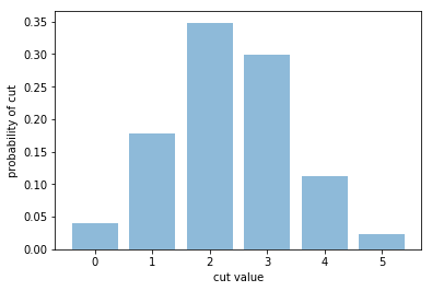
Collect the results and visualize them in a histogram¶

[4]:

# The form of the histogram has been discussed privately.
histo = simulator.GetHistogramFromCostFunction(psi, diag_cuts, max_cut);
print("The probabilities of the cut values are:")
for c in range(max_cut+1):
    print("cut={0:2d} :  {1:1.4f}".format(c,histo[c]))

# Plot histogram.
x = np.arange(max_cut+1)
fig = plt.bar(x, histo, align='center', alpha=0.5)
#plt.xticks(x)
plt.xlabel('cut value')
plt.ylabel('probability of cut')
#plt.title('Summary of results')
plt.show()

The probabilities of the cut values are:
cut= 0 :  0.0397
cut= 1 :  0.1778
cut= 2 :  0.3483
cut= 3 :  0.2986
cut= 4 :  0.1120
cut= 5 :  0.0236

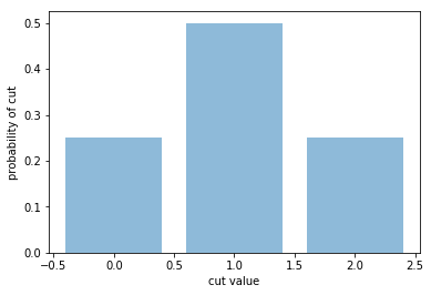
Simple test¶

This instance represents a disconnected graph with only two edges, namely: 0 – 1 2 3 4 – 5

We describe the instance by its adjacency matrix \(A\), represented as a bidimensional NumPy array.

Each of the \(2^6\) bipartitions of the 6 vertices is associated with a cut value (the number of edges connecting vertices of different color). For Half of the bipartitions the 0–1 edge can be cut and for half of the bipartitions, independently of the previous consideration, the 5–6 edge can be cut. The histogram has three bins (cut values = {0,1,2}) and ratio 1:2:1.

[5]:

# Number of vertices.
num_vertices = 6;
# Adjacency matrix.
A = np.zeros((num_vertices,num_vertices),dtype=np.int32);
# Since A is sparse, fill it element by element.
A[0,1] = 1;
A[1,0] = 1;
A[num_vertices-2,num_vertices-1] = 1;
A[num_vertices-1,num_vertices-2] = 1;

# Allocate memory for the diagonal of the objective function.
diag_cuts = simulator.QubitRegister(num_vertices, "base", 0, 0);
max_cut = simulator.InitializeVectorAsMaxCutCostFunction( diag_cuts, list(A.flatten()) );

# Number of qubits.
num_qubits = num_vertices;
# Allocate memory for the quantum register's state and initialize it to |000000>.
psi = simulator.QubitRegister(num_qubits, "base", 0, 0);

# Prepare state |++++++>
for qubit in range(num_qubits):
    psi.ApplyHadamard(qubit);

# The form of the histogram has been discussed privately.
histo = simulator.GetHistogramFromCostFunction(psi, diag_cuts, max_cut);
print(histo)

# Plot histogram.
x = np.arange(max_cut+1)
fig = plt.bar(x, histo, align='center', alpha=0.5)
#plt.xticks(x)
plt.xlabel('cut value')
plt.ylabel('probability of cut')
#plt.title('Summary of results')
plt.show()

[0.2499999999999999, 0.4999999999999999, 0.2499999999999999]

## END